Tree Searching - Class Presentation

Tree searching is essentially a method of getting from point A to point B. There are two ways to conduct a tree search: one way generates many different results at once while another locates information related to one node first. This seems confusing, but please bear with the text till the end and things may become clearer to you.

Depth-first Searching: this search method basically takes your search through a tree as far in as possible. If there aren't any "priorities", the depth first search will mindlessly delve deeper and deeper until it hits a dead end. In the picture that follows, there is a comparison of the depth-first and breadth-first search method. Take note of how even though Node A branches into several other nodes, the search only returns to it after it has reached a deadend.

Breadth-first Search: contrary to a depth-first search which ignores all other branches from a node and returns them later, a breadth-first search explores all branches from one node before moving on to another, in order of priority if such exists. Again, note the image comparing the two search methods.

(Click to see image in full-size)


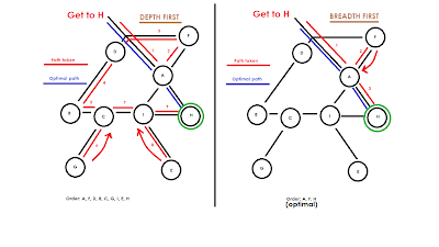
A possible application for this would be an automated maze generator/solver. Both work in essentially the same way. The program would simply randomly generate paths in a random direction and if i collides with terrain (computer limits), it will return to its previous starting point and generate in a different direction. For the maze solver, the program would explore the path uniformly until it hits a deadend and returns to the last split-point and explore the other way. In terms of mazes, the optimal search method for a solution would be the breadth-first search. Logically this makes sense because if the program chooses the wrong path, it will return to that node quicker and wind up on the right path than if it had been utilizing a depth-first search, in which case it would end up far deeper in the wrong direcion before it turns around.

This is a relatively interesting way of applying optimization that involves no calculus. In terms of mazes, we usually conduct our own breadth-first seach in our heads, mentally scanning the maze for possible dead ends and avoiding them. So get out those pencils and thinking caps!

Here's a link to an online program that demonstrates the depth-first search being utilized to "solve" a maze:

http://nullprogram.com/RunMaze/

Happy optimizing!

Optimization: Day IV - V (Lagrange Multipliers)

Today, we continued our unit on optimization problems, and worked with a new method of finding the maxima and minima of functions given a constraint: the Lagrange Multiplier.

The key to Lagrange's method is to picture the level curves of the constraint at every value, c. If the constraint is not tangent to the curve, that means there is still room to either increase or decrease the values of x and y. Naturally, by this reasoning, the maximum or minimum of the function occurs at the point(s) of tangency.

To solve a problem using the Lagrange Multiplier, gradients must be used. Take the gradient of your objective function (the function you are trying to maximize or minimize), as well as the gradient of your constraint, after moving all variables and constants to one side of the equation.

One of the key things to include, now, is the multiplier itself:

The way this is incorporated with the two gradients is the following, assuming f(x) is the objective function and g(x) is the constraint:



The reason for this can be explained by one word: tangent. When dealing with surfaces, two surfaces are considered "tangent" when their gradients are parallel. This is true when the gradient vectors are either the same, or are scalar multiples of each other. And that scalar multiple is exactly what the Lagrange Multiplier is.

The rest is simple. Distribute the multiplier into the gradient of g(x); set the x values of each vector equal to each other and solve for the multipler--do the same for the y-values.

Plug the multiplier back into the constraint, and solve for x and y. To confirm that your point is really either the maximum or minimum, choose any point that satisfies the constraint--other than the point you found--and see whether is greater or less than the function value of the point derived by the Lagrange Multiplier.

Happy optimizing!